A Self Across Time

Mark Koester

PYCON MALAYSIA, August 25, 2019

A Self Across Time
Time Series Data Analysis
with Python

Mark Koester | www.markwk.com
PYCON MALAYSIA, August 24, 2019

Slides and Code: github.com/markwk/ts4health

Slides and Code:

github.com/markwk/ts4health

Key Terms

Time Series

A time series is a sequence of observations taken sequentially in time.

George Box and Gwilym Jenkins, Time Series Analysis (2015, orig 1970)

Time Series Data Analysis

The objective of time series analysis is to decompose a time series into its constituent characteristics and develop a mathematical model for each.

Pal, D. A., & Prakash, D. P. K. S. (2017). Practical Time Series Analysis

Examples of Time Series Analysis

Financial markets: stock prices and daily closing value of the Dow Jones Industrial Average.
Natural Phenomenon: temperature trends, climate change, ocean tides, sunspots.
Economics and Price fluctations: GDP, Job Market, supply and demand, i.e. buying and selling drugs.
Health, Psychology and Behavioral Sciences: Drug or intervention analysis, investigation of natural, biological cycles

Example Time Series with Forecast Function

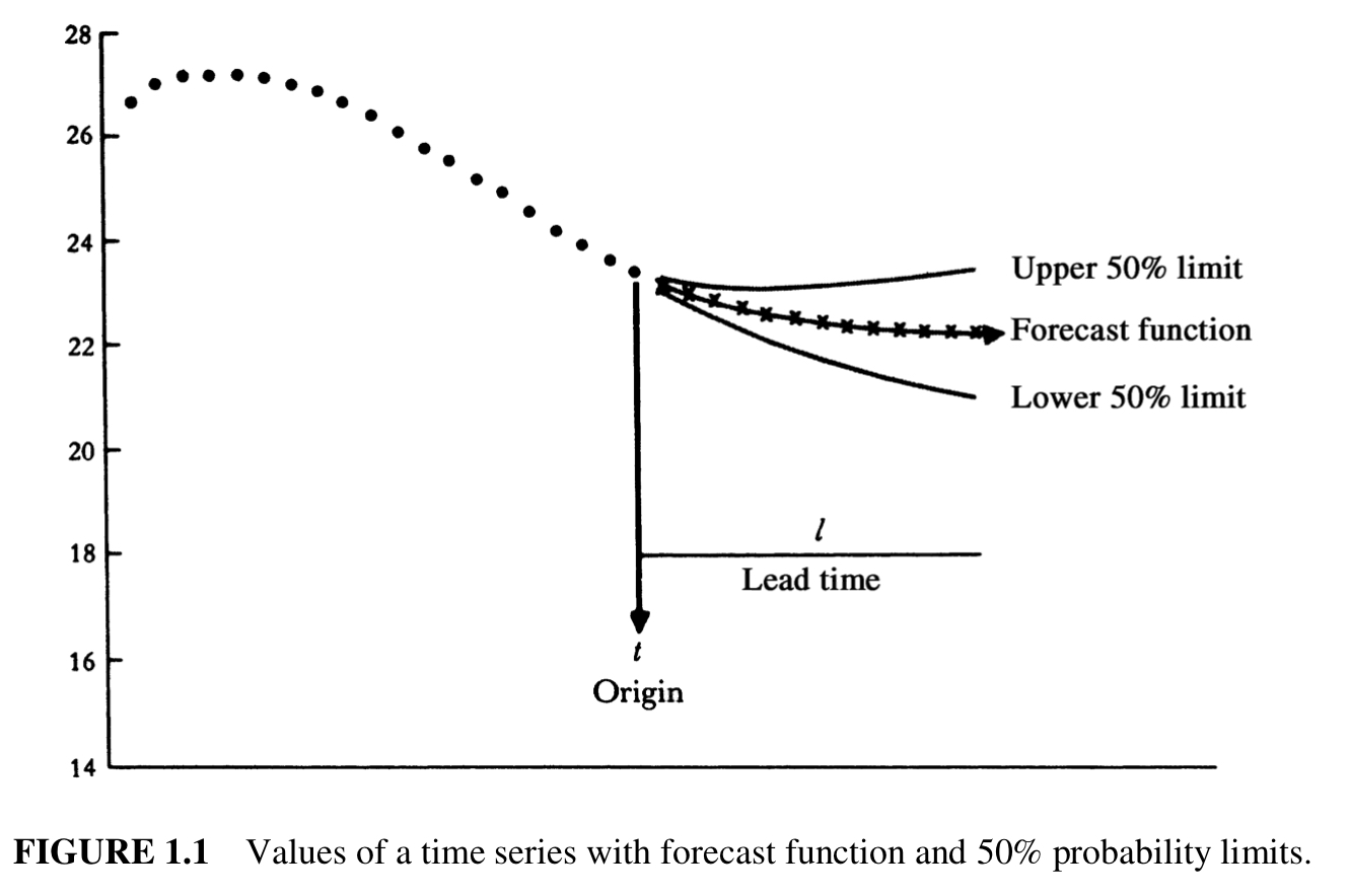
Source: Box, 2015.

Time Series Data Analysis
for Health and Self

Health: N-of-1 trials in Medical Research and Practice, esp intervention studies.
Self: Within-individual variability for Self-Trackers, Quantified Self and Biohackers.

Quantified Self (QS)

measuring or documenting something about your self to gain meaning or make improvements

Related: Self-tracking, Biohacking, Data-driven life…

Source: https://github.com/markwk/qs_mind_map

Our Question:

How to understand human health across time
or an individual self over a lifetime?

Who Am I?

deeply interesting in how both humans and technologies work
part social scientist, part technologist
software developer / builder: Int3c.com, github.com/markwk
writer / thinker: www.markwk.com, DataDrivenYou.com

My Mission

to transform science and data into better self-understanding and empowered self-improvement

Current Work

Intersection of data technologies AND human health and optimization

Doctors and companies to improve health and happiness
Quantified Self and Biohackers
Build data-driven tools with Machine Learning and AI (QS Ledger, PhotoStats.io)

A Self Across Time

Time Series Data Analysis
with Python

Talk Objectives

a conceptual understanding of time series analysis
starter code for visualizing, testing and modeling for time series effects

Talk Outline

Time and Temporal Structures of Time Series Data
Our Sample Dataset (Sleep and Exercise / Activity) and Practical Questions
Time Series Visualization, EDA, and Processing
Tests and Techniques for Time Series Data
Modeling Time Series Data
Time Series Data Analysis Applied to Health and Self
Conclusions, Next Steps and Future Directions

REFERENCES and APPENDIX

Talk Note

Focus will be on univariate, linear, discrete time series

(instead of multivariate, nonlinear, or continuous)

and assume our data/process follows a stochastic model.

Time Series Data
and Temporal Structures

What is Time?

What, then, is time? If no one asks me, I know what it is. If I wish to explain it to him who asks, I do not know.

Saint Augustine (AD 354-430, The Confessions)

Time has a pecular quality such that we think we intuitive know and understand it. But once we are asked, as Saint Augustine asked 1600 years ago, it seems rather hard to explain what we mean. In fact, some of the difficulty with defining time comes with the different perspectives we might take on the question itself. The nature of time has been a long-standing question for humans throughout history. Various philosophers, thinkers, scientists, physists and artists have all weighed in, often using their conceptual domain as the starting point.

Interestingly, while we often think of time as an innate and universal concept, when you look at history, literature and religion, you notice that our modern sense of time is a rather modern one. In fact, many earlier cultures like the Mayans did not view time as linear, as we now do, but viewed it as cyclical. According to Whitrow in various books on time, key scientific figures like Kant and Descare led to the origin of the idea of time as we know it now.

TODO: History and Evolution of Measuring Time

Timeless and the “Timed”

Much of philosophy and the history of philosophy can be thought of in terms of questions regarding what is timeless and what is not.

Much of philosophy and the history of philosophy can be thought of in terms questions regarding what is timeless and what is not. Metaphysics would be the central domain in which these questions arised, but in fact, question of what is timeless seeps into nearly all thinkers. Plato, for example, looked to the realm of the Forms to define many of his fundamental concepts. Numerous other philosophers, like Kant, depended on a timeless, immortal realm used to define ethics and reason. Hegal may have added a dynamic quality but the dialetical process transpired largely in the timeless realm of thought and outside of the empirical. Even the question of time ironically becomes whether it’s an entity and debated on the terms of metaphysics, including whether it’s real or not or just a psychological phenomenon. In short, the timeless haunts even the timed.

Two Primary Characteristics of Time:

time is unidirectional (arrow of time goes forward)
time gives order to events

Regardless of the philosophical quandries and the historical conceptions, two defining features of time stand out: 1. time is unidirectional (arrow of time goes forward) and 2. time gives order to events (Aigner, 2011). In short, “the fundamental experience of time for people seems to be events that happen one after the other” (Frank, 1998) and we often use metaphors like a river or journey to reflect this conceptualization [[201904092126_metaphor]].

General Challenges of Modeling Time

Physics of Time
Our Experience, Conception and Consciousness of Time
How do we link “models of time to people’s basic experiences”? (Frank, 1998).

Good News…

Fortunately, we don’t need to deal with these general time problems as such, because we only need to deal with the time challenges in our data!

Data Science / ML Challenges with Time Series:

How to understand the time component in a data set?
How to isolate out time…
…so we can stationalize…
…model and forecast the data?

Time Index

Time Series (general definition)

A time series is a sequence of measurements or observations that varies in time.

Time Index

Part of what happens in your data is because of the effects of time, time’s order, cycles, patterns, etc.

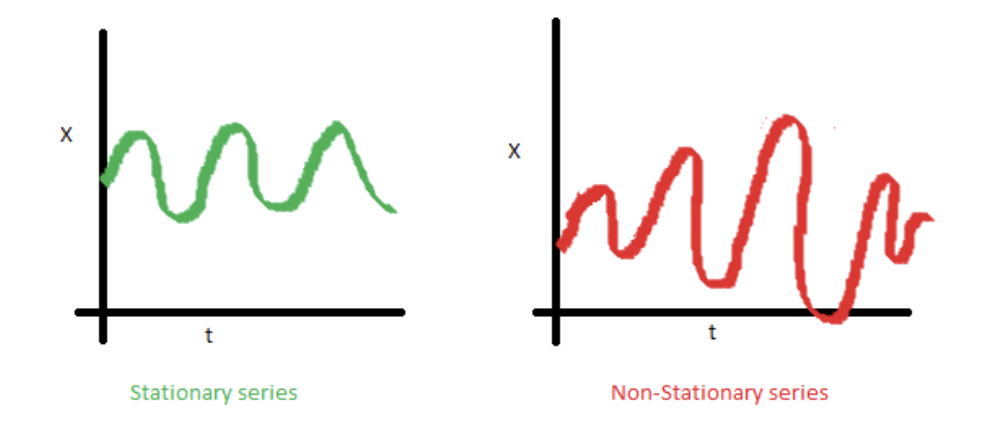
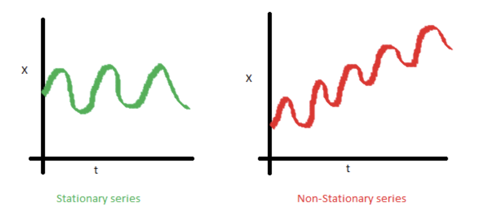
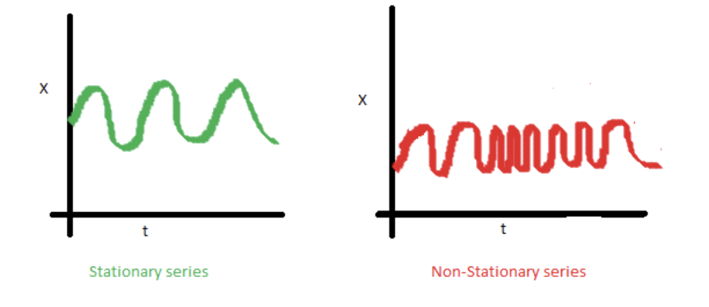
Time (Index) Can Create Non-Stationary Data

Examples of Stationary vs. Non-Stationary

Source: Analytics Vidhya

Internal Structures of Temporal Data

(aka effects of the time index)

trend (general direction of data)
seasonality (weekly, monthly, seasons, etc.)
cyclical movements (seasonality on a longer scale, often non-calendar)
serial correlation (lag, meaning previous observation(s) affect current one)
unexpected variations (noise, randomness)

Stationarity

(or stationary time series or stationary process)

Stationarity means that the statistical properties of the process do not change over time.

Why is Stationary Data Important?

Generating stationary data is important in order to understand, model, and forecast time series data.
In healthcare and biology, we need to understand if an effect is part of a trend or caused by an intervention (or other factors).

The problem with Non-Stationary Data is that it can challenging to model due to mixing of effects of time and other variables.

The main idea is that we come up with a model that makes our data regular and then once the data is regular we can use linear regression to make forecasts and see correlations outside of simply occurring along with general trends or seasonality. Practically what this means is we come up with a way to normalize the data BEFORE we model and predict. Then after during our modeling and forecasting we can then reapply the time index model to get data back into real numbers that still follow with the time index. So it’s like this 1. check if data has a temporal pattern, 2. time series model and transform the data so that temporal pattern is neutralized, 3. run actual analysis and additional modeling, 4. then apply back ts model and transformation so data is back to previous patterns.

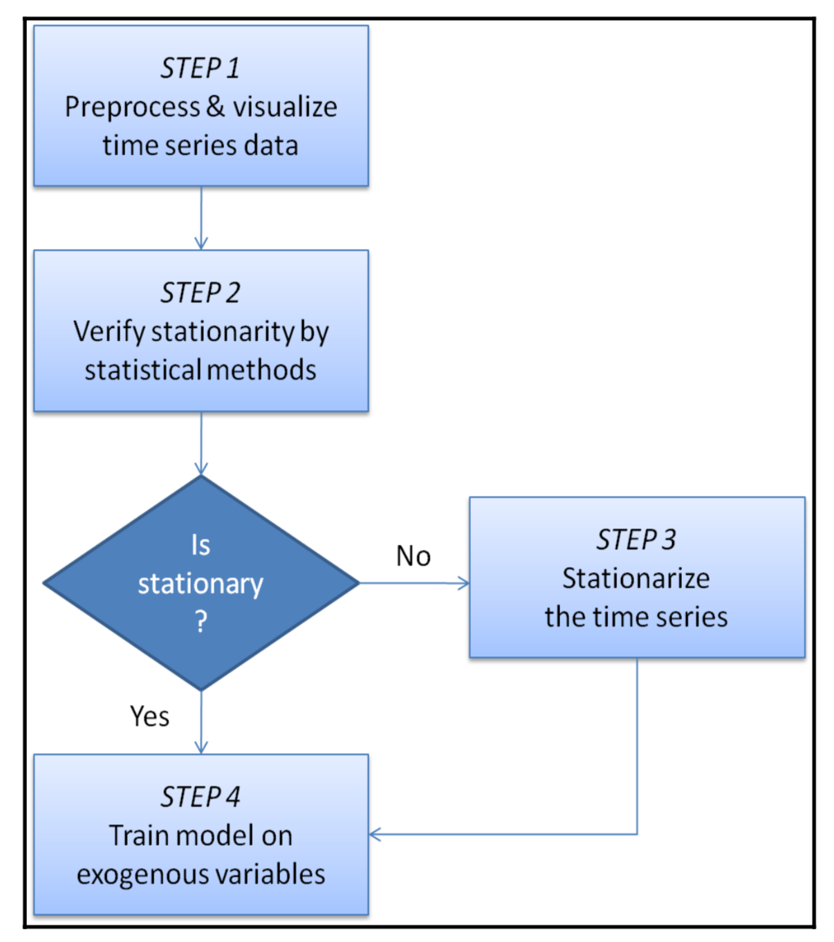
Stationarizing Our TS Data

the transformation process of decomposing and detrending ts data so non-stationary becomes stationary.

Approaches

to Time Series Data

Box-Jenkins Method

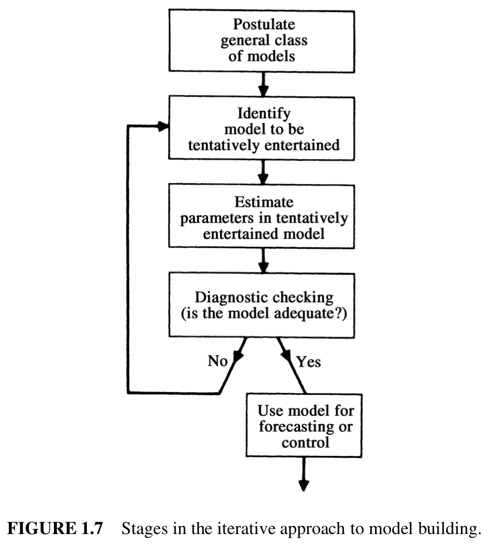
A generic methodology of time series analysis

Source: Pal, 2017.

Our Sample Dataset and Questions

Our Sample Set

Wearable Devices and individuals: Fitbit (2), Oura (1), Apple Watch (1)
Target Data:
- Sleep
- Exercise / Activity Level, inc Steps

Our Focus: Within-Individual Variablity

Practical Questions

Are there and what are the time patterns for sleep and activity levels?
Can we model and forecast these variables?

FUTURE: Does sleep correlate or affect activity level? Or vis-versa?

Data Collection and Processing

Data collection was done using a variation of QS Ledger, an open source Python project for collecting and visualization of self-tracking data (Fitbit, Apple Health, Oura, etc).
Each data set was then processed and aggregated into a standardized format.

SEE: Previous Speech Python For Self-Trackers.

Example Raw Dataset

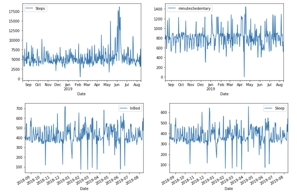
Source: Fitbit User 1

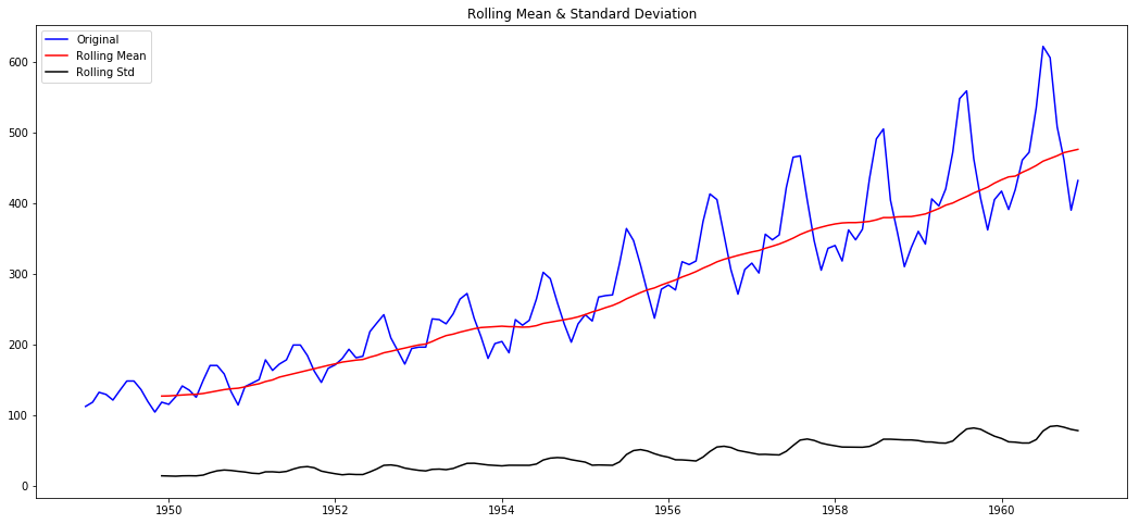
Example Data Set with Simple Moving Averages

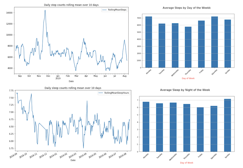
Source: Fitbit User 2

Dataset General Characteristics

Time Series Visualization

Exploratory Data Analysis

TS Data Processing

Why do we use data visualization for initial time series analysis?

check for trends, seasonality and cyclic patterns

Examples of Time Series Visualization

Line Charts
Histogram and Density Plots
Box and Whisker Plots by Interval
Heat Maps
Time Series Lag Scatter Plots

Additional Methods of Exploratory Data Analysis

Check for lag effects and scatterplot
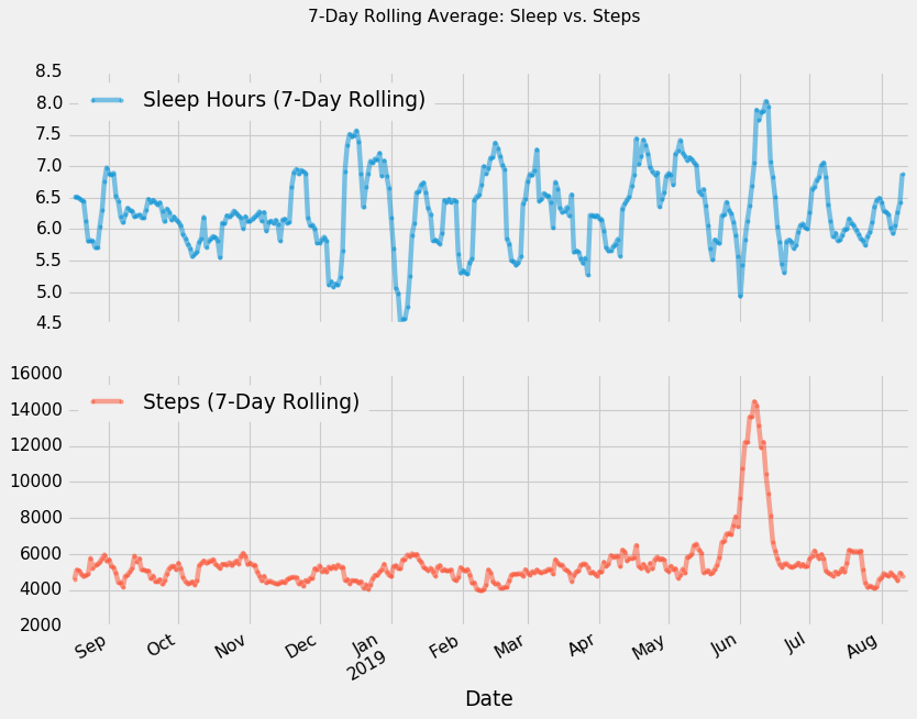
Moving Averages (i.e. rolling mean)
Exponentially-weighted moving average (EWMA)

Missing Data?

# assume zero is nan
series.replace(0, np.nan, inplace=True)

series.isna().sum()

Missing Data: Imputation

# fill in missing values if we can
if series.isna().sum() > 0:
    series = series.interpolate(method='time') # time or linear

# drops any we can't fill-in like at start of time series
if series.isna().sum() > 0:
    series.dropna(inplace=True)

Z-Scores (standard score)

Easy to calculate
Good way to compare between measurements and between individuals when scales may vary (like mood, activity, steps, sleep, etc.)

Z-Scores: Comparing Individuals

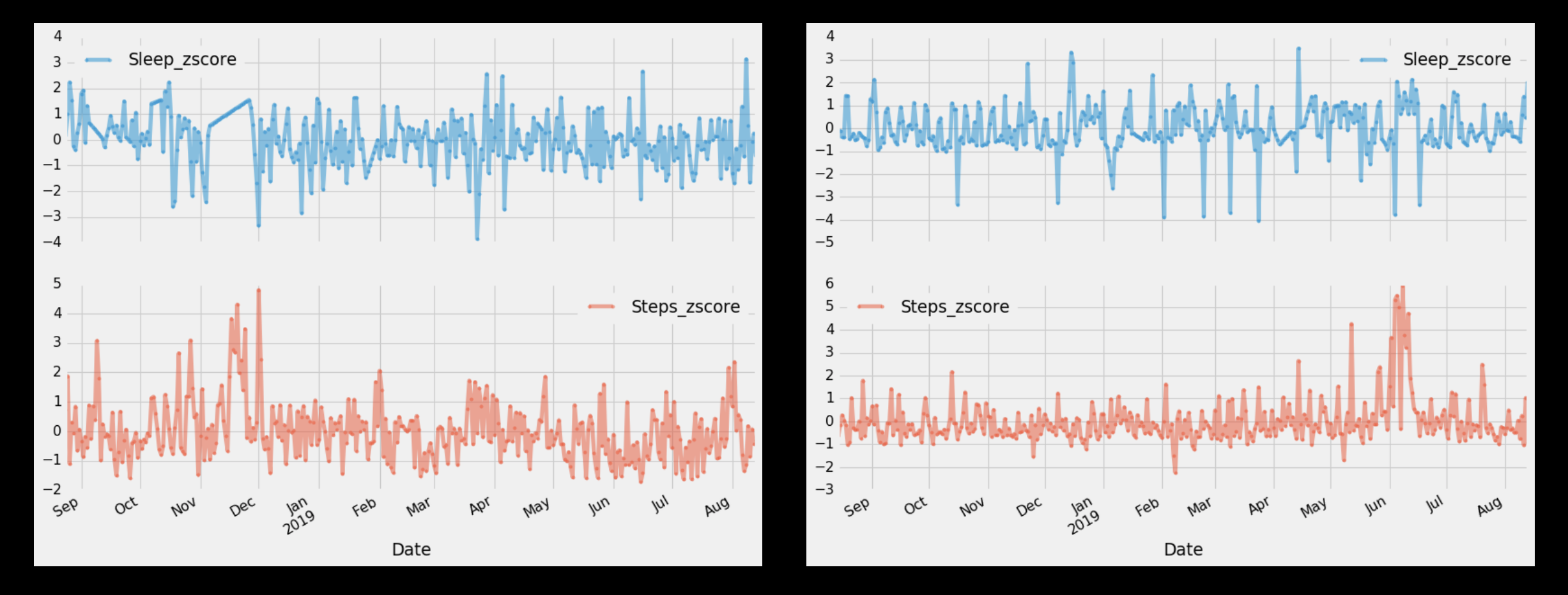
Z-Scores: Comparing Two Metrics

Z-Scores: Outlier Detection

Statistical Tests

for Detecting Temporal Effects

Statistical Tests

are used check for autocorrelation and if there are other time index effects.
Examples: Autocorrelation Function (ACF), Partial Autocorrelation Function (PACF), Dickey-Fuller Test

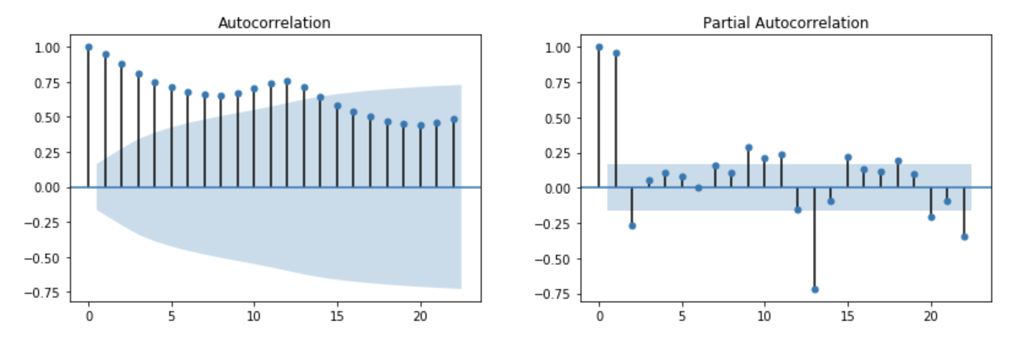
Autocorrelation Function (ACF)

ACF tells you the correlation between points separated by various time lags.

NOTE: The prefix “auto” refers to “self” (rather than automatic)

Four Sample Scenarios

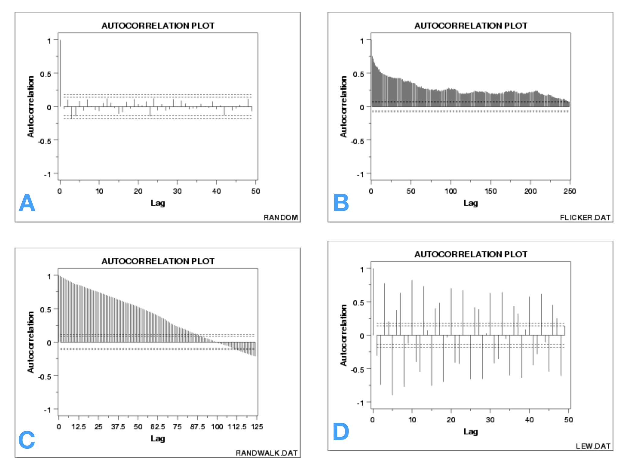
Autocorrelation Plots (Classic Pattern)

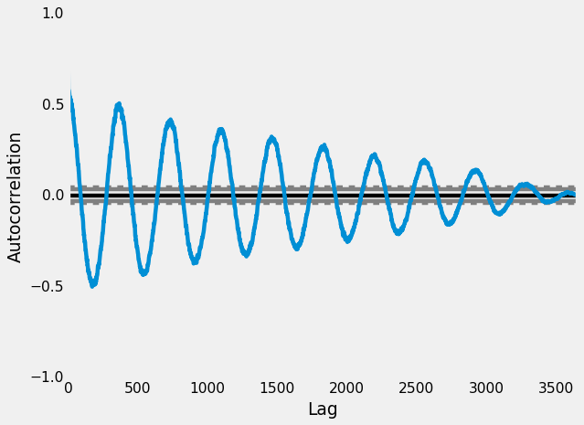
Autocorrelation Plots (Health Example)

Partial Autocorrelation Function (PACF)

shows you the relationship between an observation in a time series with observations at prior time steps but, unlike ACF, with the relationships of intervening observations removed.

CODE EXAMPLES:

Data_Visualization_Health_and_Self_Time_Series.ipynb

For background see, Time_Series_Data_Visualization_with_Python.ipynb

Code: Autocorrelation

from statsmodels.graphics.tsaplots import plot_acf, plot_pacf
plot_acf(test_ts)
# plot_pacf(test_ts)
plt.show()

Automated Dickey-Fuller Test

The Augmented Dickey-Fuller is a test used to check a univariate process or dataset for the presence of serial correlation.
The test statistic is expected to be negative. So if it is less than or more negative than the critical value we can conclude that the data is stationary.

Code: Automated Dickey-Fuller Test

from statsmodels.tsa.stattools import adfuller
#Perform Dickey-Fuller test:
print('Results of Dickey-Fuller Test:')
dftest = adfuller(timeseries, autolag='AIC')
dfoutput = pd.Series(dftest[0:4], index=['Test Statistic','p-value','#Lags Used','Number of Observations Used'])
for key,value in dftest[4].items():
    dfoutput['Critical Value (%s)'%key] = value
print(dfoutput)

Sample Scenario:

Results of Dickey-Fuller Test:

Test Statistic                   0.815369
p-value                          0.991880
#Lags Used                      13.000000
Number of Observations Used    130.000000
Critical Value (1%)             -3.481682
Critical Value (5%)             -2.884042
Critical Value (10%)            -2.578770

What Does this Mean? This data is not stationary!

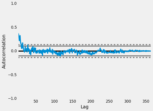
Is Our Health Data Stationary?

Autocorrelation

Apple Watch 01 Sleep

Autocorrelation

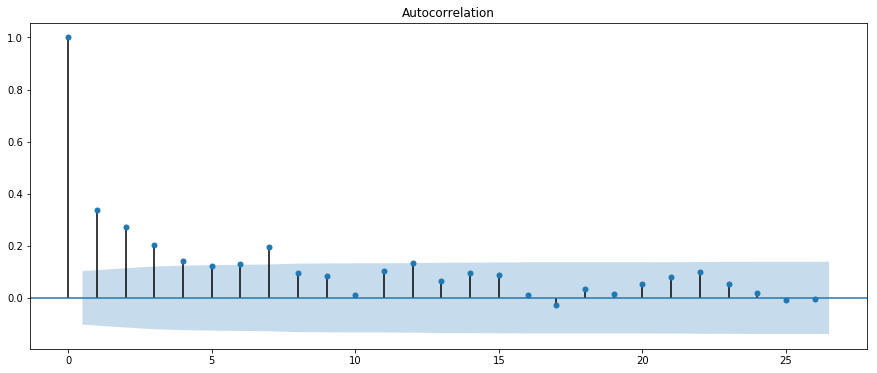
fitbit_02 Sleep

Partial Autocorrelation

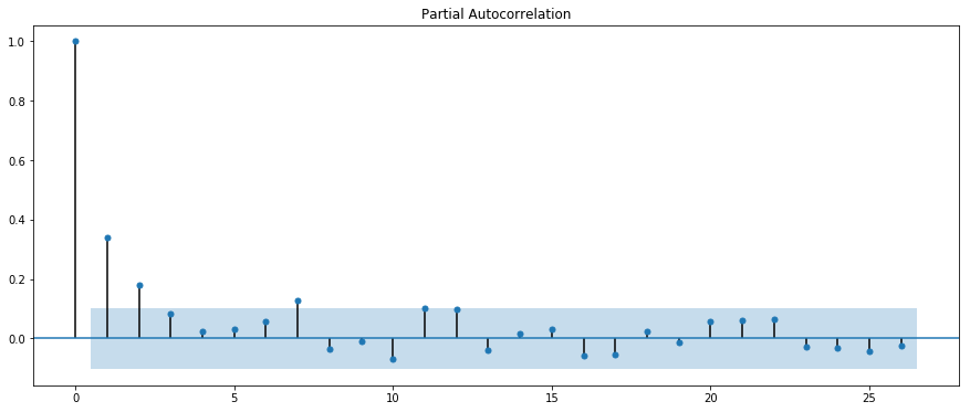
fitbit_02 Sleep

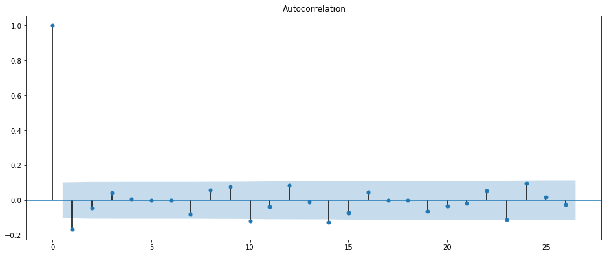
Results of Dickey-Fuller Test:

Test Statistic                  -4.625906
p-value                          0.000116
#Lags Used                       6.000000
Number of Observations Used    357.000000
Critical Value (1%)             -3.448801
Critical Value (5%)             -2.869670
Critical Value (10%)            -2.571101

fitbit_02 steps without outlier tweaking

Results of Dickey-Fuller Test:

Test Statistic                -7.57
p-value                        2.70
#Lags Used                     2.00
Number of Observations Used    3.61
Critical Value (1%)           -3.44
Critical Value (5%)           -2.86
Critical Value (10%)          -2.57

fitbit_02 steps with outlier tweaking

Steps

apple_watch_01: 
Without Averaging Out Outliers: -1.23
With Averaging Out Outliers: -7.22

fitbit_01: 
Without Averaging Out Outliers: -3.329097
With Averaging Out Outliers: -5.436158

fitbit_02: 
Without Averaging Out Outliers: -4.62
With Averaging Out Outliers: -7.57

Sleep

apple_watch_01: 
Without Averaging Out Outliers: -1.557651e+01
With Averaging Out Outliers: -19.654423

fitbit_01: 
Without Averaging Out Outliers: -5.407617
With Averaging Out Outliers:  -4.959970

fitbit_02: 
Without Averaging Out Outliers: -1.097
With Averaging Out Outliers: -4.925933

What Does this Mean?

Our health data is generally stationary.

Individual differences exist, meaning some people’s sleep or exercise numbers display more temporal patterns, like a lag effect with sleep or exercise.
Outliers can result in our data appearing more non-stationary.
By removing or averaging out outliers, we can make our data more stationary

Techniques

for Dealing with Time Series Data

Stationary TS Techniques

Smoothing: Moving average
Exponentially Weighted Moving Average
Differencing
Decomposition

TS Techniques Code:

Tests_and_Techniques_Health_and_Self_Time_Series.ipynb

Modeling & Forecasting

for Time Series Data

Box-Jenkins Model

ARIMA = Auto-Regressive Integrated Moving Average

ARIMA

AR for Autoregression: A model that uses the dependent relationship between an observation and some number of lagged observations.
I for Integrated: A preprocessing procedure to “stationarize” time series if needed, for example using differencing of raw observations
MA for Moving Average: A model that uses the dependency between an observation and a residual error from a moving average model applied to lagged observations.

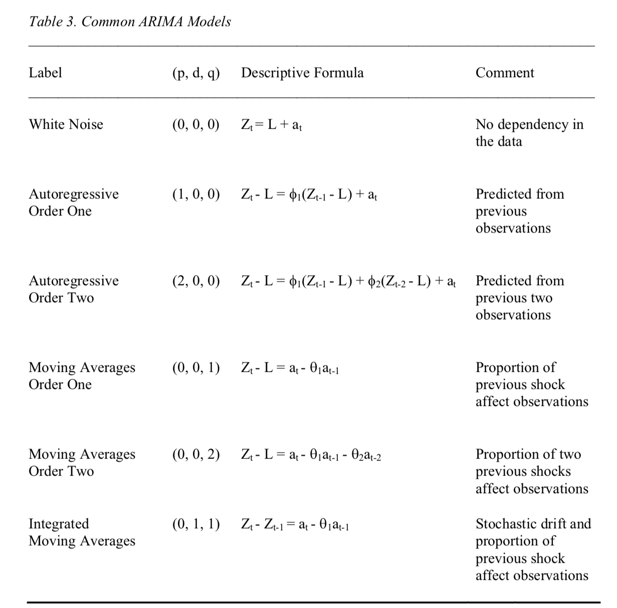
Parameters in an ARIMA Model:

Standard notation: ARIMA(p, d, q)

p The number of lag observations included in the model, also called the lag order.
d The number of times that the raw observations are differenced, also called the degree of differencing.
q The size of the moving average window, also called the order of moving average.

Common ARIMA Models

TS Modeling Code:

from statsmodels.tsa.arima_model import ARIMA
model = ARIMA(ts_log, order=(2, 1, 0)) # set parameters here
results_AR = model.fit(disp=-1)  
plt.plot(ts_log_diff)
plt.plot(results_AR.fittedvalues, color='red')

TS_Statistical_Modeling_Health_and_Self_Time_Series.ipynb

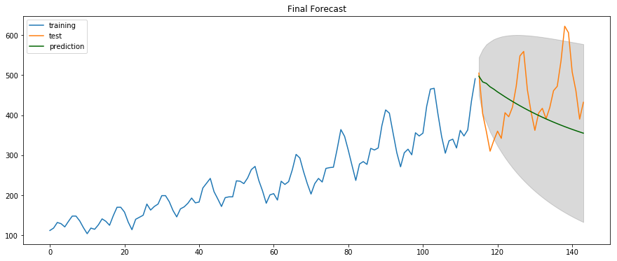
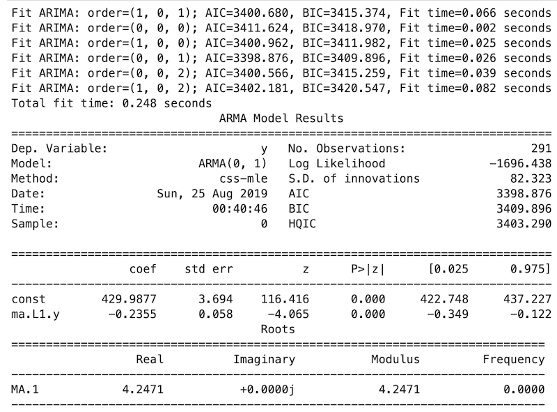
“Auto” Arima Model Selection and Forecast

Pmdarima operates by wrapping statsmodels.tsa.ARIMA and statsmodels.tsa.statespace.SARIMAX into one estimator class and creating a more user-friendly estimator interface for programmers familiar with scikit-learn.

Ref: https://pypi.org/project/pmdarima/

Auto_Arima Example:

model = pm.auto_arima(train, start_p=1, start_q=1,
                      test='adf',       # use adftest to find optimal 'd'
                      max_p=3, max_q=3, # maximum p and q
                      m=1,              # frequency of series
                      d=None,           # let model determine 'd'
                      seasonal=False,   # No Seasonality
                      start_P=0, 
                      D=0, 
                      trace=True,
                      error_action='ignore',  
                      suppress_warnings=True, 
                      stepwise=True)

print(model.summary())

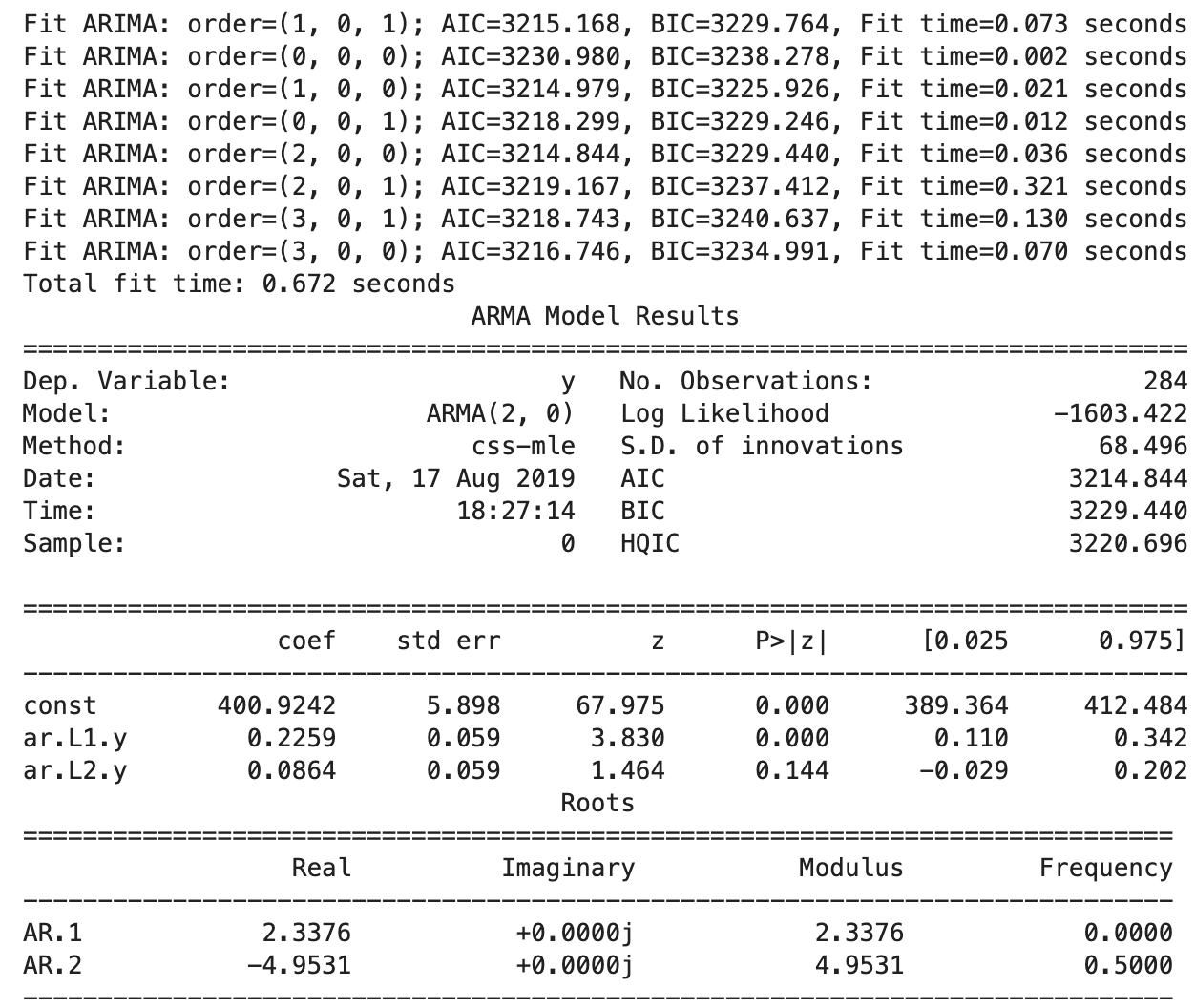
Auto_Arima Example Results:

Prophet (from Facebook)

Prophet is a procedure for forecasting time series data based on an additive model where non-linear trends are fit with yearly, weekly, and daily seasonality, plus holiday effects. It works best with time series that have strong seasonal effects and several seasons of historical data. Prophet is robust to missing data and shifts in the trend, and typically handles outliers well.

Prophet Usage 101

# pip install fbprophet

# convert to format for prophet
df.columns = ["ds", "y"]

# create and fit prophet model
m = Prophet()
m.fit(df)

Prophet Usage 101

# create empty future df
future = m.make_future_dataframe(periods=365)
# predict
forecast = m.predict(future)
# plot forecast
fig1 = m.plot(forecast)
# plot componets
fig2 = m.plot_components(forecast)

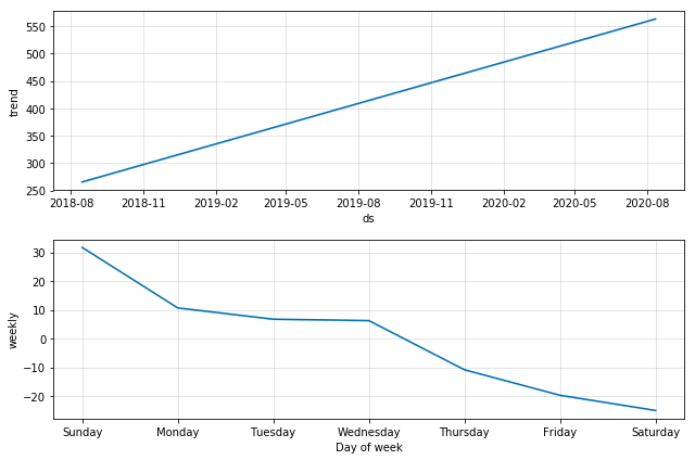
Prophet Results

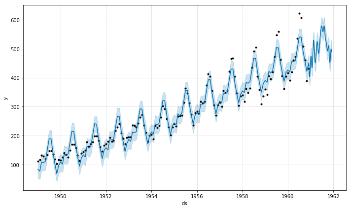
Plotting Predictions

Prophet Results

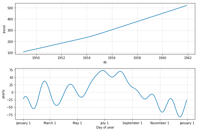
Components Breakdown

Time Series Data Analysis

Applied to Health and Self

Data Visualization

Not obvious if there are patterns or not but there are trends and up’s and downs.
Some seasonality effects (esp weekly for some individuals).
Different people sleep and move in different patterns (compared b/t self and b/t others)

Statistical Tests for Stationality

Data appears to be largely stationary but varies from person to person.
Some people have more autocollection (i.e. lag than others)

CODE: Tests_and_Techniques_Health_and_Self_Time_Series.ipynb

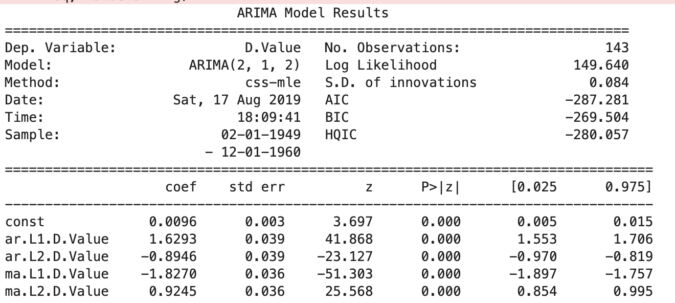
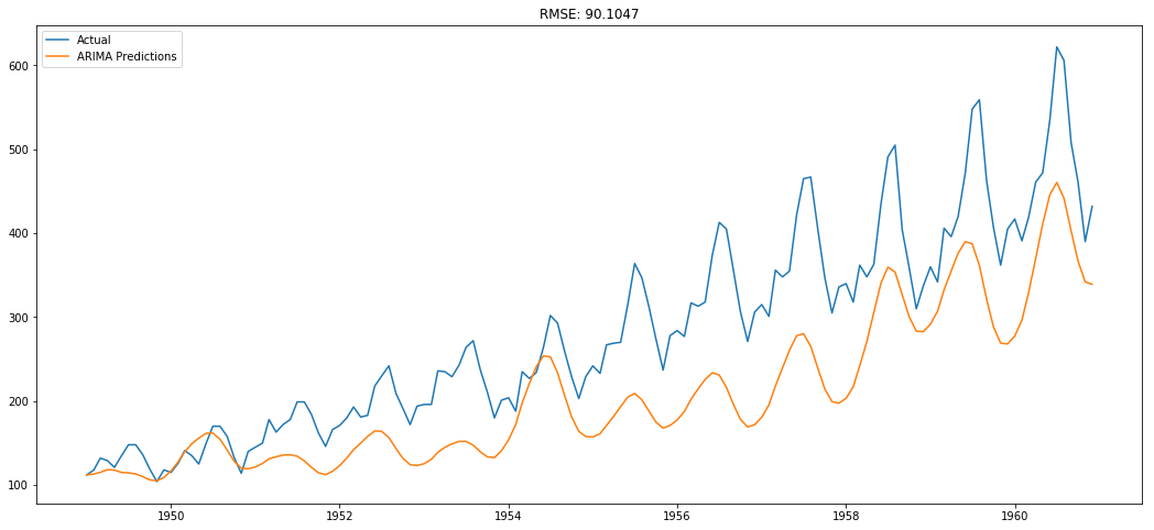
ARIMA Modeling for Health Data

Can we model the data with ARIMA?

CODE: TS_Statistical_Modeling_Health_and_Self_Time_Series.ipynb

ARIMA Modeling for Health Data

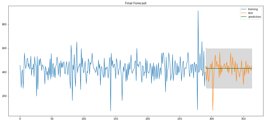
Problems with

ARIMA Modeling for Health Data

Overly sensitive to certain outliers and trends
Best model appears to be no model?

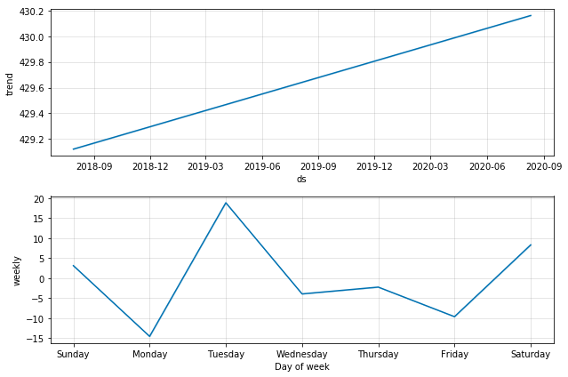
Prophet for Health Data

Can we model health data better with Prophet?

Code: Health_TS_with_Prophet.ipynb

Prophet for Health Data, Ex 1

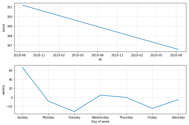
Prophet for Health Data, Ex 2

Prophet for Health Data, Ex 3

Pro’s and Con’s

Prophet for Health Data

Better at dealing with outliers
Weekly breakdown components is an interesting pattern insight
Results appear to largely be flat like better ARIMA models too
A bit of a black box model?

Conclusions

Why TS Matters, Next Steps and Future Research

Key Takeways (TS)

Temporal effects matter because unless we check for underlying trends we can’t be sure if health changes are just a temporal pattern OR caused by targetted change (like lifestyle or treatment).
Reliable statistical tests and visualizations exist to check if data is stationary.

Key Takeways (Health and Self TS)

Health data can be powerful but health patterns differ from person to person and within an individual too (and our models need to account for these).
Unfortunately numerous challanges remain for data-driven health care for doctors…
…as well as for quantified self and biohackers and little open source code exists for health and personal data analysis and modeling.

Next Steps and Future Research

Health Data World

We live in a world of devices, tracking tech and data.
It’s time to build a world of healthier selves with it.

Thanks

Slides and Code: github.com/markwk/ts4health

www.markwk.com
datadrivenyou.com

“In God we trust, all others bring data.” (W. Edwards Deming)

References

Published References

Box & Jenkins. (2015). Time Series Analysis. John Wiley & Sons. (esp Ch 1-4)
Pal. (2017). Practical Time Series Analysis. Packt Publishing Ltd. (esp Ch. 1-4)
Downey, A. (2015). Think Stats (2nd Edition). O’Reilly Media, Inc. (esp Ch 12)
Velicer. (2012). Time series analysis for psychological research. Handbook of Psychology, Second Edition. (Thorough introduction to ts for social scientists)
Aigner (2011). Visualization of Time-Oriented Data. Springer Science & Business Media.

Internet Resources 1

Time Series Data Visualization with Python - Code and example of data visualization for times series
A comprehensive beginner’s guide to create a Time Series Forecast - nice walkthrough of techniques for time series analysis and transformations
ARIMA Model – Complete Guide to Time Series Forecasting in Python - good example of ARIMA modeling with step-by-step code from analysis and parameter setting in model to forecasting and model accuracy metrics.

Internet Resources 2

Time Series Analysis with Pandas - uses Open Power Systems Data with some good examples
Pandas Time Series - pandas example using sunspots data
Playing with time series data in python - focuses on energy trends data and more deep learning methods
Working with Time Series from Python Data Science Handbook

Find me online at www.markwk.com!

A Self Across Time